Gaussian Component

pymrt.tracking.utils.GaussianComponent class implements a object class for Gaussian Component used in Guassian Mixture propagation calculation. Each Gaussian Component is defined with weight, mean vector, and covariant matrix. Methods in the class provides calculation for merging, and propagating Gaussian mixtures.

The following shows the proper usage and test case in verifying those functions.

""" This file tests Gaussian Component Calculation
"""

import numpy as np
import scipy.stats
from pymrt.tracking.utils import GaussianComponent
from mayavi import mlab


def plot_2d_gm():
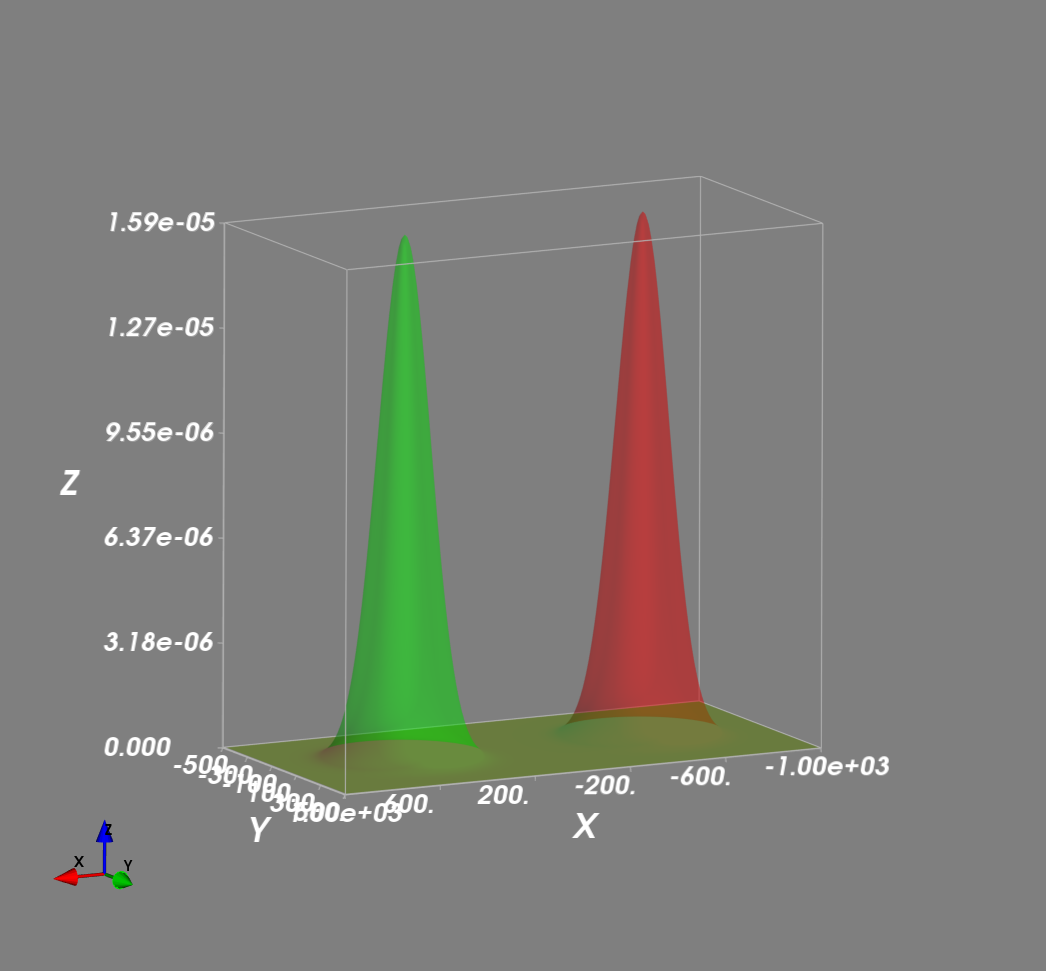
    """ This function plot two 2D Gaussian distribution density side by side
    centralized at (-500, 0) and (500, 0) for comparison.

    In this example, the Gaussian density has a covariance matrix of
    .. math::
        cov = \left[
        \begin{matrix}
        10000, 0
        0, 10000
        \end{matrix}
        \right]

    The peak of the density distribution is
    .. math::
        max(\mathcal{N}) = \frac{1}{\sqrt{2\pi 10000}} = 1.59\times 10^{-5}

    You can verify the value according to the plotted graph.
    """
    figure = mlab.figure('GMGaussian')
    X, Y = np.mgrid[-1000:1000:10, -500:500:10]
    Z_GM = np.zeros(X.shape, dtype=np.float)
    Z_PDF = np.zeros(X.shape, dtype=np.float)

    GM_mean = np.array([[-500], [0.]])
    PDF_mean = np.array([[500], [0.]])

    # Covariance matrix - with std to be 100 on both dimensions
    cov = np.eye(2) * 10000

    gm = GaussianComponent(n=2, weight=1., mean=GM_mean, cov=cov)
    mvnormal = scipy.stats.multivariate_normal(mean=PDF_mean.flatten(), cov=cov)

    for i in range(X.shape[0]):
        for j in range(X.shape[1]):
            eval_x = np.array([[X[i, j]], [Y[i, j]]])
            Z_GM[i, j] = gm.dmvnormcomp(eval_x)
            Z_PDF[i, j] = mvnormal.pdf(eval_x.flatten())

    print(Z_GM - Z_PDF)

    scale_factor = max(np.max(Z_GM), np.max(Z_PDF))
    # mlab.surf(X, Y, f, opacity=.3, color=(1., 0, 0))
    mlab.surf(X, Y, Z_GM * (2000 / scale_factor), opacity=.3, color=(1., 0, 0))
    mlab.surf(X, Y, Z_PDF * (2000 / scale_factor), opacity=.3, color=(0., 1., 0))

    mlab.outline(None, color=(.7, .7, .7), extent=[-1000, 1000, -500, 500,
                                                   0, 2000])
    mlab.axes(None, color=(.7, .7, .7), extent=[-1000, 1000,  -500, 500, 0, 2000],
              ranges=[-1000, 1000,  -500, 500, 0, scale_factor], nb_labels=6)
    mlab.show()


if __name__ == '__main__':
    plot_2d_gm()

Function plot_2d_gm() plot two 2D Gaussian distribution density side by side centralized at (-500, 0) and (500, 0) for comparison.

In this example, the Gaussian density has a covariance matrix of

\[cov = \left[ \begin{matrix} 10000 & 0\\ 0 & 10000 \end{matrix} \right] \]

The peak of the density distribution is

\[max(\mathcal{N}) = \frac{1}{\sqrt{2\pi 10000}} = 1.59\times 10^{-5} \]

You can verify the value according to the plotted graph.